Note
Click here to download the full example code
Train, convert and predict with ONNX Runtime
This example demonstrates an end to end scenario starting with the training of a machine learned model to its use in its converted from.
Train a logistic regression
The first step consists in retrieving the iris datset.
from sklearn.datasets import load_iris

iris = load_iris()
X, y = iris.data, iris.target

from sklearn.model_selection import train_test_split

X_train, X_test, y_train, y_test = train_test_split(X, y)
Then we fit a model.
from sklearn.linear_model import LogisticRegression

clr = LogisticRegression()
clr.fit(X_train, y_train)
/home/runner/.local/lib/python3.8/site-packages/sklearn/linear_model/_logistic.py:444: ConvergenceWarning: lbfgs failed to converge (status=1):
STOP: TOTAL NO. of ITERATIONS REACHED LIMIT.

Increase the number of iterations (max_iter) or scale the data as shown in:
    https://scikit-learn.org/stable/modules/preprocessing.html
Please also refer to the documentation for alternative solver options:
    https://scikit-learn.org/stable/modules/linear_model.html#logistic-regression
  n_iter_i = _check_optimize_result(
We compute the prediction on the test set and we show the confusion matrix.
from sklearn.metrics import confusion_matrix

pred = clr.predict(X_test)
print(confusion_matrix(y_test, pred))
[[10  0  0]
 [ 0 12  1]
 [ 0  0 15]]
Conversion to ONNX format
We use module sklearn-onnx to convert the model into ONNX format.
from skl2onnx import convert_sklearn
from skl2onnx.common.data_types import FloatTensorType

initial_type = [("float_input", FloatTensorType([None, 4]))]
onx = convert_sklearn(clr, initial_types=initial_type)
with open("logreg_iris.onnx", "wb") as f:
    f.write(onx.SerializeToString())
We load the model with ONNX Runtime and look at its input and output.
import onnxruntime as rt

sess = rt.InferenceSession("logreg_iris.onnx", providers=rt.get_available_providers())

print("input name='{}' and shape={}".format(sess.get_inputs()[0].name, sess.get_inputs()[0].shape))
print("output name='{}' and shape={}".format(sess.get_outputs()[0].name, sess.get_outputs()[0].shape))
input name='float_input' and shape=[None, 4]
output name='output_label' and shape=[None]
We compute the predictions.
input_name = sess.get_inputs()[0].name
label_name = sess.get_outputs()[0].name

import numpy

pred_onx = sess.run([label_name], {input_name: X_test.astype(numpy.float32)})[0]
print(confusion_matrix(pred, pred_onx))
[[10  0  0]
 [ 0 12  0]
 [ 0  0 16]]
The prediction are perfectly identical.
Probabilities
Probabilities are needed to compute other relevant metrics such as the ROC Curve. Let’s see how to get them first with scikit-learn.
prob_sklearn = clr.predict_proba(X_test)
print(prob_sklearn[:3])
[[5.28232833e-03 6.68980759e-01 3.25736912e-01]
 [9.04332610e-06 1.59729212e-02 9.84018035e-01]
 [9.86751252e-01 1.32487125e-02 3.49731273e-08]]
And then with ONNX Runtime. The probabilies appear to be
prob_name = sess.get_outputs()[1].name
prob_rt = sess.run([prob_name], {input_name: X_test.astype(numpy.float32)})[0]

import pprint

pprint.pprint(prob_rt[0:3])
[{0: 0.005282332189381123, 1: 0.6689808368682861, 2: 0.3257368505001068},
 {0: 9.04333865037188e-06, 1: 0.015972934663295746, 2: 0.9840180277824402},
 {0: 0.9867513179779053, 1: 0.013248717412352562, 2: 3.497315503864229e-08}]
Let’s benchmark.
from timeit import Timer


def speed(inst, number=10, repeat=20):
    timer = Timer(inst, globals=globals())
    raw = numpy.array(timer.repeat(repeat, number=number))
    ave = raw.sum() / len(raw) / number
    mi, ma = raw.min() / number, raw.max() / number
    print("Average %1.3g min=%1.3g max=%1.3g" % (ave, mi, ma))
    return ave


print("Execution time for clr.predict")
speed("clr.predict(X_test)")

print("Execution time for ONNX Runtime")
speed("sess.run([label_name], {input_name: X_test.astype(numpy.float32)})[0]")
Execution time for clr.predict
Average 4.41e-05 min=4.27e-05 max=5.36e-05
Execution time for ONNX Runtime
Average 1.87e-05 min=1.81e-05 max=2.34e-05

1.8663004999694978e-05
Let’s benchmark a scenario similar to what a webservice experiences: the model has to do one prediction at a time as opposed to a batch of prediction.
def loop(X_test, fct, n=None):
    nrow = X_test.shape[0]
    if n is None:
        n = nrow
    for i in range(0, n):
        im = i % nrow
        fct(X_test[im : im + 1])


print("Execution time for clr.predict")
speed("loop(X_test, clr.predict, 100)")


def sess_predict(x):
    return sess.run([label_name], {input_name: x.astype(numpy.float32)})[0]


print("Execution time for sess_predict")
speed("loop(X_test, sess_predict, 100)")
Execution time for clr.predict
Average 0.00408 min=0.00405 max=0.00415
Execution time for sess_predict
Average 0.000876 min=0.000868 max=0.000904

0.0008763897650001694
Let’s do the same for the probabilities.
print("Execution time for predict_proba")
speed("loop(X_test, clr.predict_proba, 100)")


def sess_predict_proba(x):
    return sess.run([prob_name], {input_name: x.astype(numpy.float32)})[0]


print("Execution time for sess_predict_proba")
speed("loop(X_test, sess_predict_proba, 100)")
Execution time for predict_proba
Average 0.00605 min=0.00601 max=0.0061
Execution time for sess_predict_proba
Average 0.000899 min=0.000893 max=0.00091

0.0008988612749999448
This second comparison is better as ONNX Runtime, in this experience, computes the label and the probabilities in every case.
Benchmark with RandomForest
We first train and save a model in ONNX format.
from sklearn.ensemble import RandomForestClassifier

rf = RandomForestClassifier()
rf.fit(X_train, y_train)

initial_type = [("float_input", FloatTensorType([1, 4]))]
onx = convert_sklearn(rf, initial_types=initial_type)
with open("rf_iris.onnx", "wb") as f:
    f.write(onx.SerializeToString())
We compare.
sess = rt.InferenceSession("rf_iris.onnx", providers=rt.get_available_providers())


def sess_predict_proba_rf(x):
    return sess.run([prob_name], {input_name: x.astype(numpy.float32)})[0]


print("Execution time for predict_proba")
speed("loop(X_test, rf.predict_proba, 100)")

print("Execution time for sess_predict_proba")
speed("loop(X_test, sess_predict_proba_rf, 100)")
Execution time for predict_proba
Average 0.707 min=0.705 max=0.709
Execution time for sess_predict_proba
Average 0.00104 min=0.00103 max=0.00107

0.001041621885000268
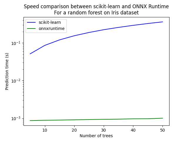
Let’s see with different number of trees.
measures = []

for n_trees in range(5, 51, 5):
    print(n_trees)
    rf = RandomForestClassifier(n_estimators=n_trees)
    rf.fit(X_train, y_train)
    initial_type = [("float_input", FloatTensorType([1, 4]))]
    onx = convert_sklearn(rf, initial_types=initial_type)
    with open("rf_iris_%d.onnx" % n_trees, "wb") as f:
        f.write(onx.SerializeToString())
    sess = rt.InferenceSession("rf_iris_%d.onnx" % n_trees, providers=rt.get_available_providers())

    def sess_predict_proba_loop(x):
        return sess.run([prob_name], {input_name: x.astype(numpy.float32)})[0]

    tsk = speed("loop(X_test, rf.predict_proba, 100)", number=5, repeat=5)
    trt = speed("loop(X_test, sess_predict_proba_loop, 100)", number=5, repeat=5)
    measures.append({"n_trees": n_trees, "sklearn": tsk, "rt": trt})

from pandas import DataFrame

df = DataFrame(measures)
ax = df.plot(x="n_trees", y="sklearn", label="scikit-learn", c="blue", logy=True)
df.plot(x="n_trees", y="rt", label="onnxruntime", ax=ax, c="green", logy=True)
ax.set_xlabel("Number of trees")
ax.set_ylabel("Prediction time (s)")
ax.set_title("Speed comparison between scikit-learn and ONNX Runtime\nFor a random forest on Iris dataset")
ax.legend()
5
Average 0.0513 min=0.0511 max=0.0517
Average 0.000868 min=0.000859 max=0.000893
10
Average 0.0862 min=0.0858 max=0.0873
Average 0.000884 min=0.000877 max=0.000902
15
Average 0.121 min=0.121 max=0.121
Average 0.000895 min=0.000888 max=0.000915
20
Average 0.155 min=0.155 max=0.155
Average 0.00091 min=0.000899 max=0.000925
25
Average 0.19 min=0.189 max=0.19
Average 0.000923 min=0.000915 max=0.00094
30
Average 0.224 min=0.224 max=0.225
Average 0.000937 min=0.000928 max=0.000956
35
Average 0.258 min=0.258 max=0.259
Average 0.000946 min=0.00094 max=0.000963
40
Average 0.293 min=0.293 max=0.294
Average 0.000966 min=0.000955 max=0.000991
45
Average 0.328 min=0.328 max=0.328
Average 0.000971 min=0.000964 max=0.000986
50
Average 0.363 min=0.362 max=0.365
Average 0.001 min=0.00097 max=0.0011

<matplotlib.legend.Legend object at 0x7f10edf70a90>
Total running time of the script: ( 3 minutes 16.934 seconds)